Score-Based Generative Models

Motivation

Given datapoints $\mathbf{x_1}, \ldots , \mathbf{x}_N$ independently¹ drawn from an underlying distribution $p(\mathbf{x})$, we would like to model the data distribution $p(\mathbf{x})$.

We can parametrize the disribution as $p_\theta(\mathbf{x})$, and try maximizing the probability of observing all data points, which is

This is equivalent to maximizing the log probability:

If we do not require $p_\theta(\mathbf{x})$ to be a valid probabilty density function (that integrates to $1$), the values of $p_\theta(\mathbf{x})$ will become arbitrarily large (and can also do so even if we impose the constraint that it integrates to $1$, depending on the parametrization). However, ensuring this density function integrates to one is typically not tractable.

Definition

The score function is the gradient of the log of the probability density function, or

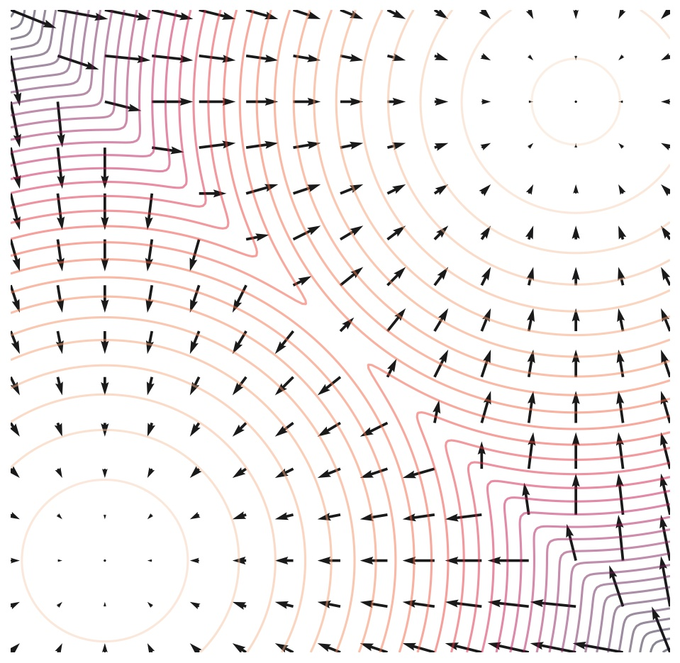
Score function of a mixture of 2 Gaussians

Avoiding the Normalizing Constant

Modeling the score function does not require knowing the normalizing constant that results in $p(\mathbf{x})$ integrating to 1.

For instance, we can model any probability distribution as \(\frac{e^{-f_\theta(\mathbf{x})}}{Z_\theta}\) Where $Z_\theta$ is a normalizing constant, which depends on $\theta$.

Taking the log of this PDF results in

And taking the gradient of this results in the second term vanishing:

The normalizing constant imposes restrictive architectural choices (like invertible layers in normalizing flows) or discretization (like outputting a softmax distribution). However, fitting $s_\theta$ does not require considering the normalizing constant, which allows for more flexibility. In fact, $s_\theta(\mathbf{x})$ only has the constraint that it should have correct input and output dimensionality, namely, both should equal the dimensionality of $\mathbf{x}$.

Optimization

We can attempt to fit the score function by minimizing

How do we know the ground truth score function? There is a technique called score matching.

Langevin Sampling

Langevin sampling allows you to sample from a distribution given its score function. First, we draw from an arbitrary distribution:

Then we iteratively perform “noisy gradient ascent”:

Where $z_i \sim \mathcal{N}(0,I)$.

As the step size $\epsilon \rightarrow 0$, and the number of steps $K \rightarrow \infty$, this will result in a sample from $p(\mathbf{x})$.

Using Langevin Dynamics to sample from a mixture of 2 Gaussians.

Instead of using the ground-truth score function, we can plug in our estimate for the score function in order to generate samples.

Additional Thoughts

Using the log allows for larger absolute scores near the edges of the Gaussian, since the numbers are smaller there, so the logarithm is large. Thus, scores are larger the further away we are from the mean of the Gaussian, which is what we want, since we want to jump further.

Adding Noise

Problems with Naive Langevin Sampling

Modeling the score function naively is difficult, because our estimates of the score function are inaccurate in low-density regions.

Note that

So the distance between the score and our estimate are downweighted in regions where $p(\mathbf{x})$ is small (low density regions). (In practice, the expectation is computed by sampling real data, so the score estimate is inaccurate where we have little data).

This complicates Langevin sampling, since $\mathbf{x}_0$ (the first sampling step) usually starts in a low-density region according to the data distribution (it is usually just noise).

Additional Thoughts

Adding two random variables

1. Recall from Brad Osgood’s course that adding two random variables $Z = X + Y$ results in a distribution that is a convolution of the distributions of $X$ and $Y$.

2. By adding noise to our data, we are essentially smoothing the data distribution with a gaussian kernel.

3. This smoothing can be thought of as increasing the support of the distribution. Think about it - if we add lots of noise, almost anything can arise with some probability.

4. In addition, we can represent our data distribution as a set of discrete samples, or impulse functions at each datapoint. The sifting theorem means that the noisy data distribution can be represented as a mixture of Gaussians.

Score function of a Gaussian

1. Note that the score function of a Gaussian is linear:

1. In fact, if we consider the Gaussian distribution as originating from a data point at $\mu$ with added noise $n \sim \mathcal{N}(0,\sigma^2)$, then we have that a sample $x$ from the Gaussian is:

And the score function is

That means that the score function is proportional to the noise added!

Score function of Mixture of Gaussians

1. The score function of a mixture of gaussians is approximately piecewise linear. It would be exactly piecewise linear if our smoothed distribution was piece-wise Gaussian. In a mixture of Gaussians, there is some spillover from other Gaussians everywhere.

2. Since ReLU neural networks output piecewise linear functions, they are great for modeling score functions. (This was from Mert’s class)

Improved Score Matching

Adding lots of noise corrupts the data distribution substantially, while adding low levels of noise may not result in enough smoothing or coverage. We can choose $L$ levels of noise:

We can compute the noisy distributions:

Additional Thoughts

Interpreting the Integral

We can view computing this integral like this:

1. Iterate through all possible data examples $\mathbf{y}$
2. Compute the probability that $\mathbf{x}$ occurs under a normal distribution centered at $\mathbf{y}$.
3. Sum across all possible values of $\mathbf{y}$, weighted by the data distribution $p(\mathbf{y})$.

Expectation

This can also be viewed as an expectation:

Or, when we sample $\mathbf{y}$ from our data distribution $p(\mathbf{y})$, what is the expected density of a normal distribution centered at $\mathbf{y}$?

Convolution

Note that this can be seen as the convolution between two probability distributions:

Where

Flipped Convolution

Since convolution is commutative, there are two ways to express a convolution, and we can also express it as

In this case, we integrate over all possible values of the normal distribution $q$, and evaluate $ \mathbf{x - y}$ (or equivalently $\mathbf{x + y}$, since adding noise subtracting noise do the same thing) according to the data distribution.

Basically, there’s a different way to “add up” to $\mathbf{x + y}$, one for each value of $\mathbf{y}$ sampled from a normal distribution. We’re essentially accumulating across all these possible ways to “add up” to $\mathbf{x}$. We can also express this as an expectation:

Which is saying, draw a sample (noise) from the normal distribution, and evaluate the probability of the data distribution at the point where example that results from subtracting that noise.

In other words, $\mathbf{y}$ is the noise added to the data example $\mathbf{x}$, and we are evaluating $p(\mathbf{x})$ according to the data distribuition, but we are aggretating over all possible noises that could have been added, which is $\mathbf{y}$.

We can also think of this as fixing the noise vector, and asking, “What is the probability density if the noise is this?” Then we accumulate over all possible noise vectors.

End Additional Thoughts

Drawing samples from $p_{\sigma_i}(\mathbf{x})$ is easy, we can just draw a sample $x \sim p(\mathbf{x})$ from our dataset and add noise to get $\mathbf{x} + \sigma_i \mathbf{z}$.

We can fit a neural network to the score function of each noisy distribution:

The training objective is:

Usually, the loss weighting is $\lambda(i) = \sigma_i^2$. This would mean higher noise levels have a greater loss.

The ground truth score estimates are usually $\frac{-\mathbf{z}}{\sigma}$

We can run Langevin dynamics in sequence for each noise level. This means runnning Langevin chains for all noise levels.

Recommendations

We can choose the noise levels in a geometric progression (there is a common ratio). $\sigma_L$ can be the maximum pairwise distance between two datapoints, and $L$ can be hundreds or thousands.

Next steps

As $L \rightarrow \infty$, the noise level becomes a continuous-time stochastic process, where noise is added. This will allow for generative modeling using SDEs.

Last Reviewed: 2/4/25